Introduction
Jupyter notebooks are really useful interactive coding environments that bring along documentation capacity in readable, non-code format. This means we can use Jupyter notebooks to develop and test code and legibly explain what’s happening all in the same place. So far so good; and there are lots of great videos online showing this environment in action.
If you would like to build a Jupyter notebook environment (a notebook server) on a cloud machine: You’re in the right place. The directions here are “from the ground up” and serve a second purpose as well, which is (we at CloudBank hope) to de-mystify building on and using the cloud.
Before we begin, however: Remember that cloud providers like to do things for us “as a service”. You can get into Jupyter notebooks in this manner in Azure or on the Google Cloud Platform or on Amazon Web Services or on the IBM Cloud etcetera. If you choose to go this way there are two things to check on: The cost for the value-added service and whether the results of your work will be transferable to other environments / platforms.
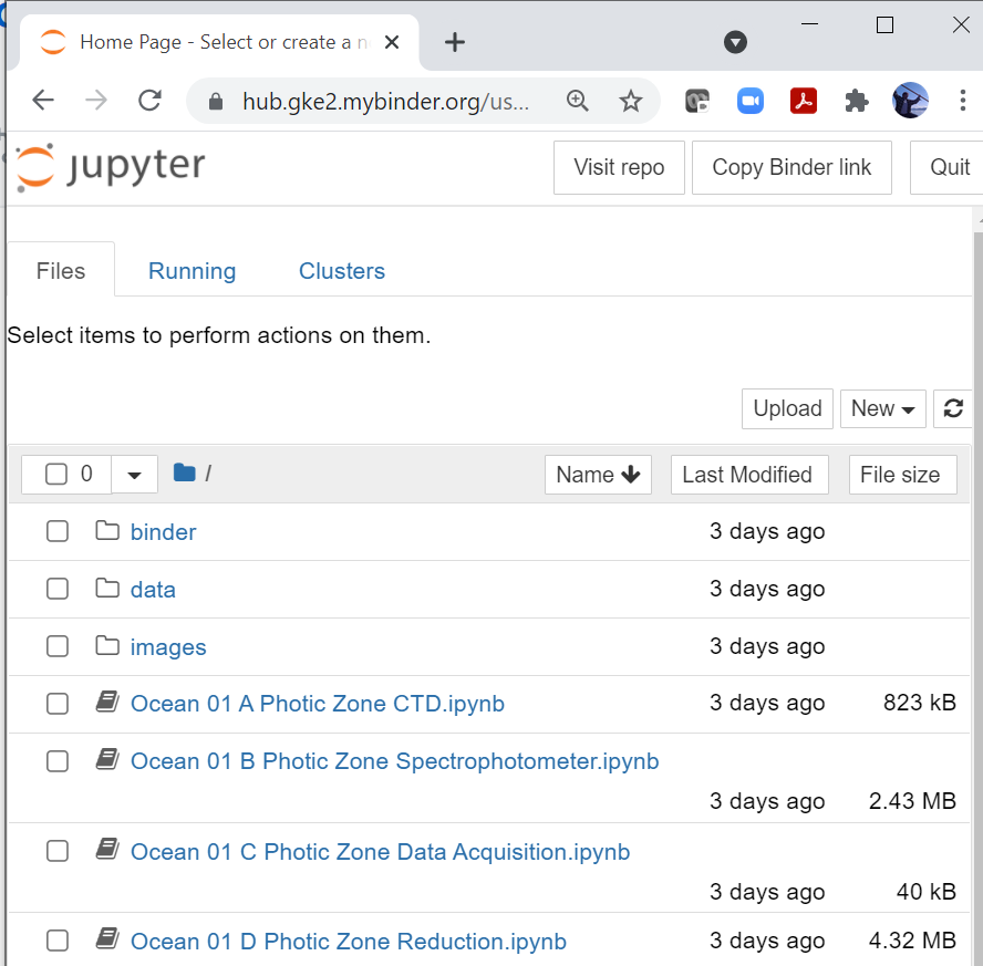
That said, we’ll proceed with the Do It Yourself On The Cloud approach. Here is an example of a notebook server browser interface.
What is the plan?
Learning to compute on the cloud includes understanding machine images:
Snapshots of an entire operating system including installed software, customization,
code and data. This CloudBank solution serves two purposes: It introduce machine images
and it demonstrates using a cloud virtual machine (herein VM) as a traditional desktop--possibly
quite a powerful one--for running a Jupyter notebook server.
The interface to this working environment will be via a web browser on our Local machine.
We move information back and forth securely from Local to Cloud using an ssh tunnel.
Why instructions are necessary
At a high level we are configuring a research computer. Because it is on the cloud there is some extra vocabulary involved and some extra steps, starting with securing a cloud account. There is enough complexity to merit a walk-through. Here’s the narrative:
A researcher decides to work on the public cloud; and gains access...
Cloud access agreements commonly are called ‘accounts’ or ‘subscriptions’
CloudBank uses the term billing account
Using a browser interface the researcher starts a dedicated cloud VM and logs in
The researcher configures the VM as a Jupyter Lab notebook server supporting a Python kernel
Other useful tools / libraries / packages / datasets are installed
The researcher tests the Jupyter Lab server by connecting via browser
This makes use of a secure connection called an ssh tunnel
The researcher uses cloud management tools to create an image of the VM on the cloud
Unlike a container, this image is cloud-specific (not transferable to other clouds)
The researcher Terminates (deletes) the VM: It is no longer available
The stored image persists and can be used to start up a new VM
A VM may be in one of two states: Started or Stopped. We pay for a VM by the hour: Only when it is Started. Stopped is like having the power turned off: You can resume using it later without loss of data. Terminating a VM means the VM no longer exists: Everything is gone.
Starting a VM from an image recreates the machine in its state when the image was created. When you do this you have a choice of which type of VM to use for the image. You can use a cheap low-power VM if you do not need a lot of computing power; say you just want to write and test some code. Or you can choose a powerful (more expensive) VM if you have some heavy computation to do.
Notice that you may start many VMs from a single image. Your collaborators may use an image to start their own VMs as well. This means that customized work environments are easy to replicate and share.
Key concepts
Authentication
Authentication is “logging in”, i.e. you are authenticated to use a resource on the cloud
On the cloud there are (at least) three authentication paths: Username/password, login keypairs and IAM Access Keys
Authentication is generally credential use over a secure connection
The secure connection is built into applications like ssh as a protocol: It just works.
The credential may be a file containing long text strings: Guard as if they are passwords to your bank account
Cautionary tale: An Access Key file for your cloud account can be used to automatically run tasks
This means that someone with your access key can easily spend $15,000 in one hour mining bitcoin
Do not place credentials on Virtual Machines that will be used to create images per this walk-through
Virtual Machines (VM / VM instance / “EC2” on AWS, “Google Compute Engine” on GCP, “Azure VM” on Azure)
Wide variety of instance types to choose from.
Any given instance type will have associated memory, processing power and storage (see below).
The cost of the instance -- per hour -- varies with these characteristics.
On the AWS console you select the EC2 service and then Launch Instance
This runs a launch wizard: First step is to choose an operating system image
Second step is choose instance type
Search on
cost <instance-type> <cloud provider>to check rate per hour
Block storage is the term used for a disk volume: Root operating system, data drives etc
On AWS this is called Elastic Block Storage (EBS)
AWS also supports temporary disk storage through the instance store
Distinguish between Elastic Block Storage (EBS) and (ephemeral) instance store volumes
Instance store volumes evaporate on Stop/Start. EBS volumes persist through Stop/Start.
Additional storage modes:
AWS EFS (Elastic File System) shared by multiple instances; ~ UNIX NFS
Walk-through
Again these use AWS as the “example cloud” but these notes will apply broadly to any cloud. The short version describes what to do with scant attention to specifics. The extended version is more comprehensive.
Short version
Install a bash shell on your Local computer (laptop, desktop etc)
Start a cloud VM, note three things:
the generic VM username (here we use
ubuntu)the ip address of the VM (here we use
12.23.34.45)download the key pair file to Local (here we use
keypair.pem)
Assign the VM a stable (static) ip address
This ip address does not change even when you stop and re-start the VM
AWS: Use the Elastic IP service. GCP and Azure: The term is static external IP.
chmod 400 keypair.pemandssh -i keypair.pem ubuntu@12.23.34to log in to the cloud VM from LocalFrom the command line on the cloud VM install
miniconda,jupyterand other Python librariesUse
git clone https://github.com/organization/repositoryon the cloudNeed a working example? Use organization =
cloudbank-project, repository =ocean
On the VM: Start a Jupyter Lab notebook server as a background process with browser display disabled
Example command to listen on port 8887:
(jupyter lab --no-browser --port=8887) &Note the token string printed by the Jupyterlab start-up process
On Local: Create an
sshtunnel associating Local port 7005 with VM port 8887Example ‘ssh -N -f -i keypair.pem -L localhost:7005:localhost:8887 ubuntu@12.23.34.45’
On Local, in a browser address bar: Enter
localhost:7005and at the prompt enter the token stringThis connects to the Notebook server on the cloud VM via the ssh tunnel
Test out some notebook functionality; verify that the Python kernel runs etcetera
Stop and re-start the VM and again test functionality
Stop the VM and create an Amazon Machine Image (AMI)
Terminate (delete) the VM
Re-start the VM from the saved image and again test functionality
Note that the development of code within a
gitrepository supports back-ups and collaborationA VM to be used for extended time (days or longer) is a candidate for a daily auto-Stop
On AWS: CloudWatch and Lambda functions are commonly used for this purpose
This action prevents charges from accruing overnight when the VM is not in actual use
Use the AWS console to make the VM machine image (AMI) available to other people
Extended version
Log on to the AWS console and select Services > Compute > EC2 > Launch Instance
This may also be done with the Command Line Interface (CLI) for AWS or using an API such as
boto3
Run through the launch Wizard; here are some details by example:
Image: 64 bit x86 Ubuntu Server (username =
ubuntu): Bare machine image, just the OSVM:
m5ad.4xlarge, cost $1.00 / hour in Oregon at time of writingThis instance type includes two 300 GB instance store volumes (temporary storage)
Data on these volumes is temporary, will evaporate: Don’t put anything important here
Remember to Stop or Terminate this instance once you start it (and know the distinction)
Zombie resource charges happen when we forget about a VM that keeps running
Configure instance: Default values
Make the root volume larger (say 100GB) to create some working space
Add Tags: Added key values
Name,Project,Date,Owner, etcetera as appropriateConfigure Security Group: Default values
Review and Launch: Create a keypair file
keypair.pemand download it to LocalLaunch: Note resulting ip address of the VM; let’s say it is
12.23.34.45
From my own computer log on to the AWS EC2 instance
Relocate the downloaded keypair file to my
bashhome directorychmod 400 keypair.pemis a permissions change applied to the keypair fileConnect with the vm:
ssh -i keypair.pem ubuntu@12.23.34.45
On the EC2 instance (VM) mount any added storage drives
Search engine: 'AWS EC2 EBS mount` gives this instructive link
Install the Jupyter Lab notebook serve
Install Anaconda or Miniconda
search
install Anaconda Linuxand follow the instructionsOnce the download path is determined I used
wgetto download the installer on the VMwget https://repo.anaconda.com/archive/Anaconda3-2020.07-Linux-x86_64.sh
On Ubuntu I installed in the
/home/ubuntudirectory and needed to add the path forcondaexport PATH=~/anaconda3/bin:$PATH
Once Anaconda is installed: use the
condapackage manager to install Jupyterlabconda install -c conda-forge jupyterlab
Configure the machine for research
Install software packages
The following are example installation commands (geoscience-oriented)
conda install xarrayconda install -c conda-forge cmoceanconda install botoconda install netcdf4conda install -c conda-forge ffmpegconda install networkxpip install utmsudo apt install nodejsworking towards widgets...
Import datasets:
sftp -rfrom the data directory of a data source computerrequirements.txtorenvironment.yml:pip freezeand related links needed
Create an image (AMI) of this Virtual Machine
On the AWS console: EC2 'running instances table: Locate and select this instance
When you run the Create Image process the VM will be Stopped
Actions menu > Image > Create Image
Be sure to attach extensive metadata (typically add Tags) to the AMI to make it recognizable
Share the AMI with other AWS accounts
On the AWS console > AMI listing (see left sidebar) > Permissions editor
Add the AWS 12-digit account of a destination account where you wish this AMI to be available
Terminate the VM
This step established that it is safe to Terminate a VM backed up by a machine image
Do this as a proof of concept operation
WARNING: This will completely delete this EC2 instance
You could Start a new EC2 instance from the AMI prior to the Terminate just to be careful
You can verify everything is preserved as you expect in this new instance
At this point the AMI has been demonstrated as correct and you can Terminate both EC2 instances
On the AWS console > EC2 ‘Running Instances’ table: Locate and select an instance to Terminate
Actions menu > Instance State > Terminate and confirm
Notes
Once per month updates is a typical pace
Update the operating system:
sudo yum updateCreate a new AMI and manage your AMI catalog to avoid zombie AMIs
On the VM:
ps -ef | grep jupyterto see if the server is runningjupyter nbextension enable --py widgetsnbextension
left off here
what follows is a copy paste of the original student hands-on for restoring and using a VM. As such it can be reduced down to a much smaller section here.
CloudBank Solution Repo: Research Computing and Cloud Images
This tutorial introduces you, the researcher or student, to using a virtual machine image
on the cloud as a basis for research computing. This page describes using an image
that has already been built for you. If you want to see how to do the preparatory
build: Look into the creating_an_image sub-folder.
You may be familiar with a zip or tar file containing an entire directory. A machine image is analogous; think of it as a zip file of the entire computer’s contents from operating system to home directory to code to data files. The idea is that once a cloud Virtual Machine (VM) is configured for use: It can be stored as a machine image. This image is then un-packed back onto a Virtual Machine. The image is used to creating a working research computing environment for a scientist to use.
Our specific example here takes advantage of the Jupyterlab notebook server. This page
is a tutorial for going from a pre-built Linux environment with Jupyterlab installed
as an image and reconstituting it on the AWS cloud as a Virtual Machine. We will use
a secure tunnel called an ssh tunnel to enable you the researcher to connect to the
Jupyterlab server through your web browser.
In the sub-folder called bootstrap we go through the process of building this machine image.
In the sub-folder called waterhackweek we go from the rebuilt Jupyterlab VM to cloning a
repository of notebooks on the VM for a particular research topic.
Important remark on cost management
In what follows on this page: The VM has a single disk drive (filesystem) with a fairly small
capacity of 32 Gigabytes. However it is common practice to create images that bundle large
datasets. The sub-folder bootstrap tutorial spins up a Virtual Machine, for example, that has
200 GB of block storage (disk drive) volume mounted as two data filesystems.
This allows the image builder to include a moderately large dataset with the image
and provide some working space as well.
Our point of emphasis here -- as with all cloud resource allocation actions -- is that one should understand and track the costs associated with cloud resources. ‘Block’ or ‘disk’ storage -- for example -- runs about $20 per month for 200 GB.
Again our main admonition: The cloud is very powerful but it is important to understand and manage the cost of using it.
Outline
In what follows please customize your resources by substituting your own name for
hedylamarr.Obtain credentials to log in to the cloud console: Contact cloudbank for details
Identify the proper image and use it to jumpstart a Virtual Machine instance
Log on to this instance and start up a Jupyter Lab server
Create an ssh tunnel from your computer to this server
Use your browser to connect to the Jupyter Lab and use this to explore some data
For Windows Users
A brief interruption anticipating a possible issue: Further down we are going to build something called an “ssh tunnel” to use our Virtual Machine as a Jupyter notebook server. If you are doing this on a PC running Windows: No problem, that’s perfectly feasible but Windows does not natively make this Linux-y step trivial. So be ready: We will introduce the idea of installing a small Linux bash shell on the Windows PC. It is a bit of a “yet another step, really??” situation but on balance it can help save time and avoid frustration. Instructions are here.
Connecting to a Jupyterlab server built on a cloud Virtual Machine
Suppose we would like to visually explore some (ocean) data. This data took years to collect and months to bring together in one location. Hopefully it takes less than an hour to deploy and connect to a Jupyterlab notebook server on the cloud.
Prerequisites: Cloudbank credentials to connect to the cloud and an available
bashshell.
We are using in this case the AWS (Amazon Web Services) cloud. You will log on to the AWS console, start a Virtual Machine (called an EC2 instance) and on that machine start a Jupyterlab server. If you were starting from nothing you would be installing Python packages and importing datasets. Our objective here is to avoid all of that by using a pre-built environment stored on the cloud as an image. Once you have identified this image you can start it on virtually any size machine; from a small cheap one say costing 2.40 / hour or more. Cloud users choose a computer based on computational needs.
Once the computer is running (with everything pre-installed) you will create an ssh tunnel. This is a secure connection that associates a local address on your local comoputer with the Jupyterlab server running on the cloud VM. By connecting through this tunnel the cloud VM becomes the backing engine for exploring the data.
The procedure is presented in 13-or-so steps with interspersed comments. Upon completion you will have your own data science research environment.
Procedure
Log on to the AWS console using your credentials; and be sure to set your Region (upper right drop-down) to Oregon o Sidebar: You can choose Services (upper left) to see a listing of services, i.e. what you can do on the AWS cloud
Navigate to Amazon Machine Image choices (AMIs): Services > Compute > EC2. Then choose AMIs from the left sidebar.
In the upper left drop down menu of the AMI pane select ‘Private Images’ (it may say ‘Owned by Me’ or ‘Public Images’ by default). When ‘Private Images’ is selected, you should see an AMI listed called
jupyter1-cb. Select this AMI by clicking on it so a blue dot appears at the left edge of the table.Choose Actions > Launch. Choose a VM type
c5.large(you may have to scroll down a bit to find this). Choose Review and Launch at the bottom right.
WARNING: If this tutorial is a class-sized activity there is a potential collision scenario. Let’s take a moment to outline this and how to resolve it.
The AWS EC2 Launch Wizard goes through seven steps. Step 6 involves choosing a Security Group. This SG is given a name by default; and a classroom full of people will get the same default as they proceed. So the way to avoid this (which will obstruct the next couple of steps) is to click on the Security Group step (step 6) and give a name for the Security Group that is unique. As below with keypair and instance names the best choice for a Security Group name is simply
yourname. In our instructions we use the namehedylamarras an example of your name. Now you can proceed to step 7 of the wizard; which is step 10 in this procedural.
Choose Launch at the bottom right. In the ensuing keypair dialog choose Create new keypair and name it
hedylamarr. This will be the key to identifying your instance and logging in to it in what follows. Download the keypair file you generated; then click Launch Instance in the dialog box.Continue in the AWS console: Click View Instances at the lower right. This takes you to a table of EC2 instances (Virtual Machines), where one instance is listed per row. Therefore one of the rows in this table should be your instance.
Class strategy remark: You now have a Virtual Machine (“EC2 instance”) on the public cloud. If you are in a class with many people doing the same thing at the same time it can be difficult to identify which instance is your VM. Once you identify your instance: Name it using
yourname.
Locate your instance by the key name: In the table of instances scroll right to find the
Key namecolumn. Scan down this column for the keypair you used to identify the row for your EC2 instance. Return to the left-most Name column of this row -- the row for your instance -- and hover your cursor to bring up a pencil icon in the “Name” column. Click on that and name your instance appropriately.One the instance status dot changes to green (running): Note its
ip addressin the instance table. Here we take this to be12.23.34.45as an example.
Now we are ready to log in to this VM or EC2 instance from a bash shell. Our main goal on the instance is to start a ‘quiet’ Jupyterlab session. There will not initially be a browser interface; that comes a little further down. Once the Jupyterlab server starts it will print a token, a long string of letters and numbers used to authenticate; so be prepared to copy that to a text editor for a few minutes.
On your computer: Open a
bashshell and ensure the keypair filehedylamarr.pemis present in your working directory. Issue achmodcommand to give the keypair file limitedrwxpermissions:chmod 400 hedylamarr.pem.
If running Windows on your local computer: You may need to install or enable the native
bashshell. As an alternative you can install an Ubuntubashshell. In either case it is useful to realize that the home directory of this shell is not the same location as the Windows User home directory. Ifhedylamarr.pemwas downloaded toC:\\Users\hedylamarr\Downloads: Move it to yourbashhome directory, for example using this sequence of commands:
bash> mv /mnt/c/Users/hedylamarr/Downloads/hedylamarr.pem ~
bash> cd ~
bash> chmod 400 hedylamarr.pem
The
sshcommand insists the authentication keypair filehedylamarr.pemhave User read-only permission, Files in the Windows User area are not amenable tochmod; so we relocate this file and proceed inbashfrom~. These details can very frustrating so we go to the trouble to elaborate this here.
In bash run
ssh -i hedylamarr.pem ubuntu@12.23.34.45to connect to your EC2 instance. (Use the correct ip address.) Respondyesat the prompt to complete the login. Note that your username isubuntuand you have the ability to run root commands usingsudo.
If you have configured the image using (for example) the tutorial in the
bootstrapsub-folder: You may wish to spend some time looking around to ensure the instance is configured as expected. For example if there are additional data disks you can check to see these have been mounted properly.
On the command line of your EC2 instance issue
(jupyter lab --no-browser --port=8889) &After about one minute this command should produce multiple lines of output including atoken string.
...token=ae948dc6923848982349fbc48a2938d4958f23409eea427
...token=ae948dc6923848982349fbc48a2938d4958f23409eea427
Copy this string to a text editor for later use.
If you lose this token just log on to the instance where it is running and issue jupyter notebook list to see it.
Issue exit to log out of your cloud instance.
Note: The Linux structure
(command) &causescommandto run as a background job. This allows you to log out of your instance, leaving it to function as a Jupyterlab server.
Note: The above token is used the first time connecting to the Jupyterlab server. It may not be used in subsequent sessions but it is worth keeping it around. If it is lost for some reason: Re-start the Jupyterlab server on the VM and re-copy the token.
In the
bashshell issuessh -N -f -i hedylamarr.pem -L localhost:7005:localhost:8889 ubuntu@12.23.34.45. (Make appropriate substitutions.)
This
sshcommand creates an ssh tunnel to the EC2 instance running the Jupyterlab server. You associate a location on your own computer (localhost:7005) with the connection point on the EC2 instance (12.23.34.45:8889). The number trailing the colon, called a port, acts as a qualifier for the connection.
In your browser address bar type
localhost:7005. This should change tolocalhost:7005/lab?. When prompted for the token paste in the token string you copied earlier. You should now see a Jupyterlab environment. When using the instructional image for this tutorial there should be a notebook listed on the left calledchlorophyll.ipynb. You may click on this notebook to open it and explore the contents.
Idiosyncratic Cloud Notes
To add a “data disk” to the VM allows us to create and manage additional storage capacity on a VM
These persistent drives are called Elastic Block Storage (EBS) volumes on AWS
AWS EC2 VMs may also feature instance store volumes equivalent to
/tmpstorage: Nothing persists here.
Updating Anaconda and the machine image operating system
Once per month is a common Anaconda update tempo...